on
Effect of the Economy on the Election (Week 2)
Introduction
The aim for this week’s blog post is to understand the force, if any, that economic variables have on the election. Our understanding of the presidential election is largely shaped around the election. Researchers Christopher Achens and Larry Bartels have found that economic growth, particularly in the last quarter before the election, is highly correlated with the success of the incumbent president (Achen and Bartels, 2017). This model of voting assumes that the voter is rewarding or punishing the president for their ability to manage the economy, but that they’re slightly myopic and don’t take into account the whole term. Below, we’ll explore whether this is also the case for House elections, as well as dive deeper into the usage of an economic model to predict House elections.
Economic Indicators
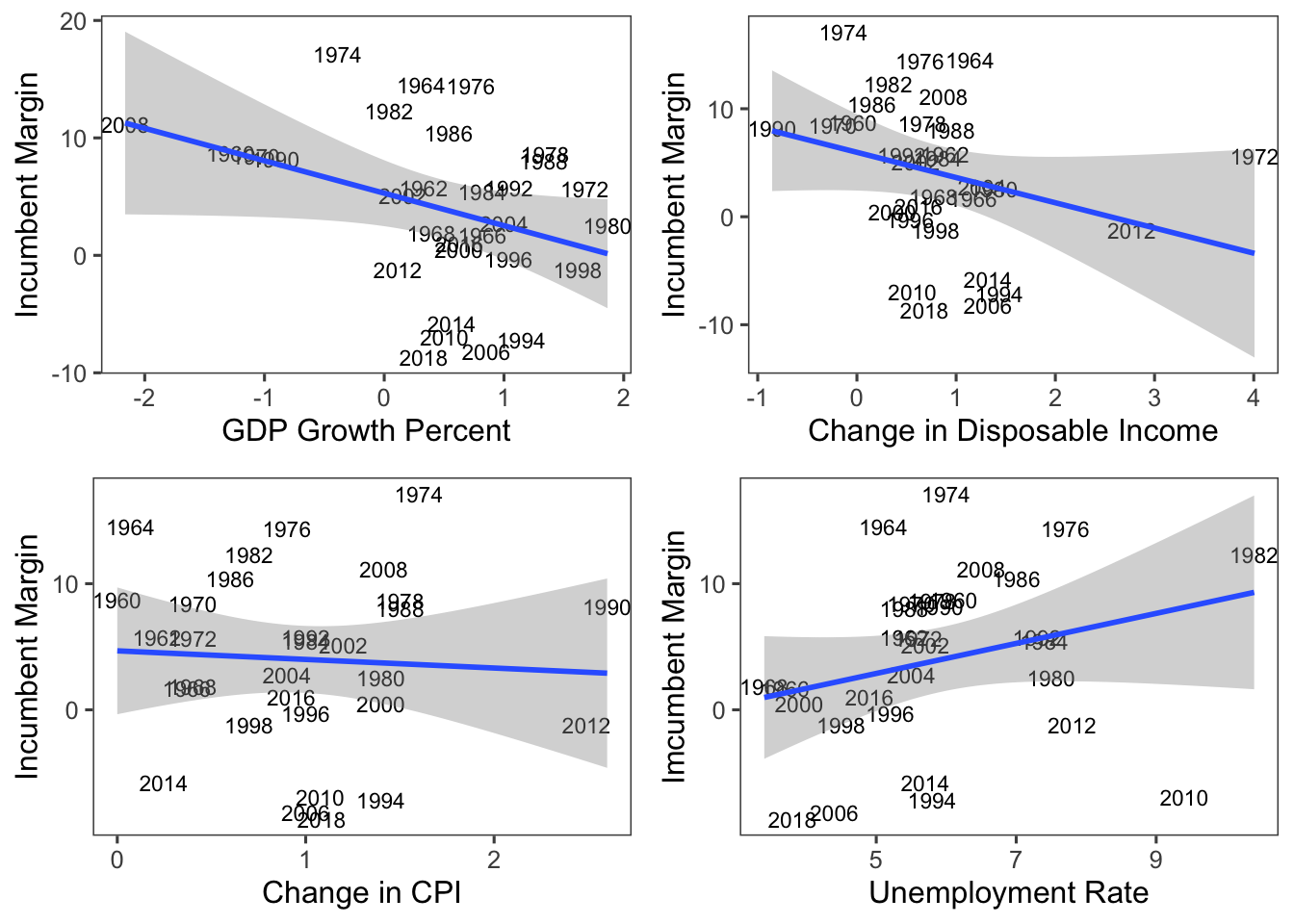
First, we examine the relationship between various economic variables and the success of the incumbent party in House elections:

From these, we can see that there appears to be a non-zero relationship between incumbent margin and GDP growth percent, change in disposable income, and unemployment rate. It is important to note, however, that there are notable outlier years that are driving the relationship, and that in many years, these variables fall within one percent of each other. Going forward, this will need to be adjusted for.
Building a Model with Year in Mind
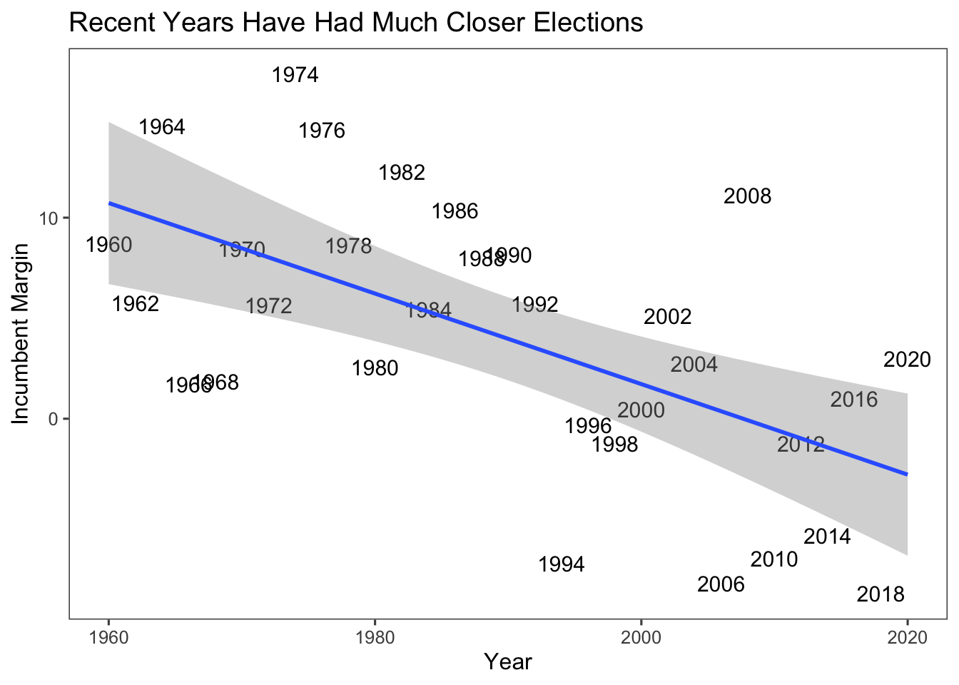
In exploring various economic variables, I realized that there was a very strong relationship when I inputted the base economic variable (for example CPI instead of change in CPI). This eventually led me to realize that it was because these variables almost consistently grew over time, meaning that time itself was an important factor in the prediction of incumbent margin. Below, I’ve plotted incumbent margin’s relationship to the year the election was in, and here we can see quite a strong negative relationship, where recent elections have had a much lower incumbent margin. A potential theory for why elections are getting closer is gerrymandering or other electoral law changes, or simply a narrowing of the vote. Either way, this relationship is not one to be ignored.
## Warning: The following aesthetics were dropped during statistical transformation: label
## ℹ This can happen when ggplot fails to infer the correct grouping structure in
##   the data.
## ℹ Did you forget to specify a `group` aesthetic or to convert a numerical
##   variable into a factor?
In a basic linear model, we find that while economic variables struggle to explain incumbent margin, with the slight exception of GDP growth percent, it seems that year is highly explanatory.
##
## ==========================================================================
##                                           Dependent variable:
##                               --------------------------------------------
##                                             incumbent_margin
##                                 (1)      (2)      (3)     (4)      (5)
## --------------------------------------------------------------------------
## GDP_growth_pct                -2.694*
##                               (1.319)
##
## DSPIC_change_pct                        -1.593
##                                        (1.217)
##
## cpi_change                                      -0.636
##                                                 (1.798)
##
## UNRATE                                                   1.164
##                                                         (0.776)
##
## year                                                            -0.225***
##                                                                  (0.056)
##
## Constant                      5.315*** 5.156*** 4.640** -2.981  452.012***
##                               (1.347)  (1.519)  (2.262) (4.793) (112.385)
##
## --------------------------------------------------------------------------
## Observations                     31       31      31      31        31
## R2                             0.126    0.056    0.004   0.072    0.354
## Adjusted R2                    0.096    0.023   -0.030   0.040    0.332
## Residual Std. Error (df = 29)  6.544    6.800    6.983   6.742    5.625
## F Statistic (df = 1; 29)       4.168*   1.713    0.125   2.249  15.895***
## ==========================================================================
## Note:                                          *p<0.1; **p<0.05; ***p<0.01
Final Model Construction
The final model that I use is a multiple linear regression model with all four measures of the economy laid out above: GDP growth percent, change in disposable income, change in CPI, unemployment rate, and the year of the election. This is shown below as model number 2, and has an adjusted r-squared of 0.505, meaning that this model explains 50.5% of the variation in incumbent margin.
##
## ==================================================================================
##                                          Dependent variable:
##                     --------------------------------------------------------------
##                                            incumbent_margin
##                              (1)                   (2)                 (3)
## ----------------------------------------------------------------------------------
## GDP_growth_pct             -1.656                -1.742               -2.076
##                            (1.075)               (1.035)             (1.387)
##
## DSPIC_change_pct           -1.023                -0.984               -1.286
##                            (0.988)               (0.963)             (1.290)
##
## cpi_change                  1.706                 2.053               -1.680
##                            (1.756)               (1.577)             (1.827)
##
## UNRATE                     1.098*                1.040*               1.175
##                            (0.597)               (0.575)             (0.771)
##
## year                      -0.251***             -0.268***
##                            (0.073)               (0.057)
##
## winner_partyR              -0.940
##                            (2.600)
##
## president_partyR            1.499
##                            (1.804)
##
## Constant                 495.693***            530.436***             0.700
##                           (144.044)             (113.220)            (4.963)
##
## ----------------------------------------------------------------------------------
## Observations                 31                    31                   31
## R2                          0.602                 0.587               0.226
## Adjusted R2                 0.481                 0.505               0.107
## Residual Std. Error    4.958 (df = 23)       4.841 (df = 25)     6.503 (df = 26)
## F Statistic         4.967*** (df = 7; 23) 7.121*** (df = 5; 25) 1.897 (df = 4; 26)
## ==================================================================================
## Note:                                                  *p<0.1; **p<0.05; ***p<0.01
It was an easy choice to choose this model over that of model 3, which includes just economic variables, because model 3 has much lower explanatory power with an adjusted r-squared of 0.107. Choosing model 2 over model 1, however, took a bit more leg work. Model 1 adds control variables for which party won and the party of the president in the year of the election. Thoughts on the election may lead us to add these - it seems important who won the election and who is currently in power - but these variables play out badly in the model. I found this by working to find the best model for the incumbent margin of each variable size through the comparison of adjusted r-squares, as shown below.
##          GDP_growth_pct DSPIC_change_pct cpi_change UNRATE year winner_partyR
## 1  ( 1 ) " "            " "              " "        " "    "*"  " "
## 2  ( 1 ) " "            " "              " "        "*"    "*"  " "
## 3  ( 1 ) "*"            " "              " "        "*"    "*"  " "
## 4  ( 1 ) "*"            " "              "*"        "*"    "*"  " "
## 5  ( 1 ) "*"            "*"              "*"        "*"    "*"  " "
## 6  ( 1 ) "*"            "*"              "*"        "*"    "*"  " "
## 7  ( 1 ) "*"            "*"              "*"        "*"    "*"  "*"
##          president_partyR
## 1  ( 1 ) " "
## 2  ( 1 ) " "
## 3  ( 1 ) " "
## 4  ( 1 ) " "
## 5  ( 1 ) " "
## 6  ( 1 ) "*"
## 7  ( 1 ) "*"
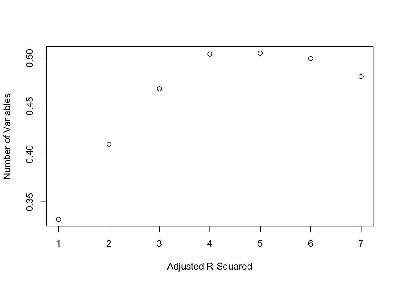
What this tells us is that, of these seven variables, were we to try to make the best model we can out of five variables, we should exclude the winning party and the president’s party variables from the analysis. I further confirmed that the control variables should be removed by plotting the adjusted r-squareds of different numbers of variables in the model. We can see below that adding the sixth and seventh variable to our model only decrease the explanatory power of the model, thus we choose model 2.

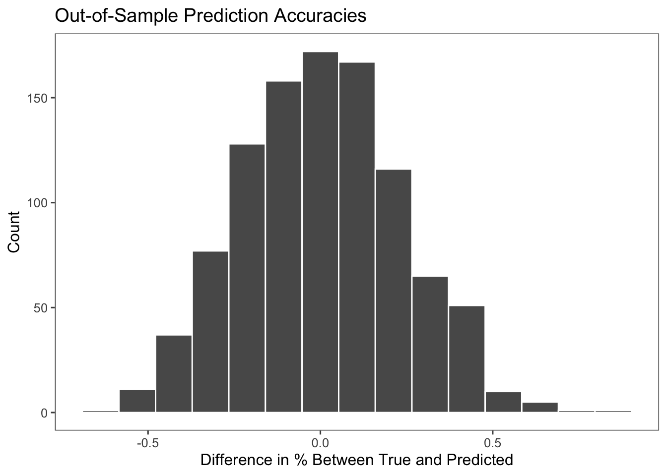
This method that we’ve used to optimize the model, however, can be dangerous. Especially since we have quite a small number of data points, precisely choosing the best variables can lead to overfitting of the model such that it fails outside of the sample. In order to counteract this, I use cross-validation to ensure that this model is not overfit by removing a random sample of 8 of the 31 elections to keep as test data. The graph below shows the difference between the true incumbent margin and predicted incumbent margin of 1000 cross-validated samples. Error is approximately normally distributed around zero, and the majority of the mean error falls between 0.5% and -0.5% which indicates that the model is acceptable.

Conclusion
While this is not a perfect model by any means, it does take a first stab at attempting to predict the House election using economic indicators. Using this model, we get the following prediction based off of current economic indicators:
##          fit       lwr      upr
## 1 -0.9529354 -7.114136 5.208266
This means that the verdict of the economic model is that the incumbent margin will be -0.95%, meaning that Democrats narrowly lose the House by two-party vote-share. It is important to note, however, that the lower and upper bounds for this point prediction are quite wide and indicate much uncertainty about the final victor. Future work will be needed to predict the House race wth greater certainty.