on
Adding Turnout to District-Level Predictions (Week 6)
Introduction
This week we examine the ground game by campaigns. Campaigns are primarily occupied with persuading voters to vote for them and turning out people that already support them to vote. We looked at persuasion last week through television ads, but for this week, we’ll be examining the turnout factor instead. Academic literature has found that having field offices in a county increase that county’s vote-share by about 1% in the 2008 election (Darr & Levendusky, 2014). In addition, we learned from the 2012 election that campaigns have the potential to increase voter turnout by up to 8% points (Enos & Fowler, 2016). This means that in order to understand the ground game in each district, we can explore differences in turnout in each district and incorporate that into our model of the election.
Turnout Model
To investigate turnout, I begin by building an election forecast district-by-district. I use variables that have been found to be important in past weeks - the national generic ballot, the percent difference in GDP from Q6 to Q7, and incumbency. To this, I add the district-level voter turnout, which is found through adding Republican and Democratic votes and dividing by the citizen voting-age population (CVAP). We use these variable to predict the democratic two-party vote-share in a district. I use this model specification for all 435 districts. Below is an example of this model for one district (Wyoming).
| Example Regression Model | |||
| Wyoming | |||
| Characteristic | Beta | 95% CI1 | p-value |
|---|---|---|---|
| average_support | 1.3 | -16, 19 | 0.5 |
| turnout | 0.09 | -3.9, 4.1 | 0.8 |
| gdp_percent_difference | -0.38 | -4.5, 3.7 | 0.4 |
| incumb | |||
| Adjusted R² = -0.544; No. Obs. = 5 | |||
| 1 CI = Confidence Interval | |||
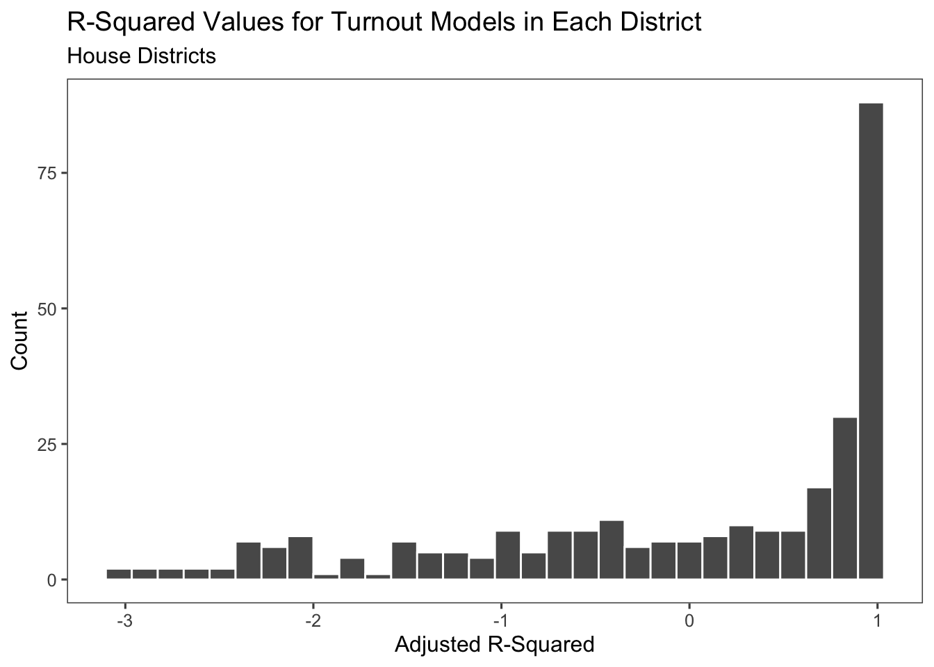
From this Wyoming model, we can see a number of issues already. This model is not great - none of the variables are significant, the adjusted r-squared is negative, and incumbency is all the same, and thus is not regressed on. Most of the issues stem from the fact that there are only five observations in this model since we only have five years worth of turnout data due to the redistricting cycle. Below, we can take a look at the adjusted r-squared across all 435 models - we can see that this model tends to be quite bad across the districts.
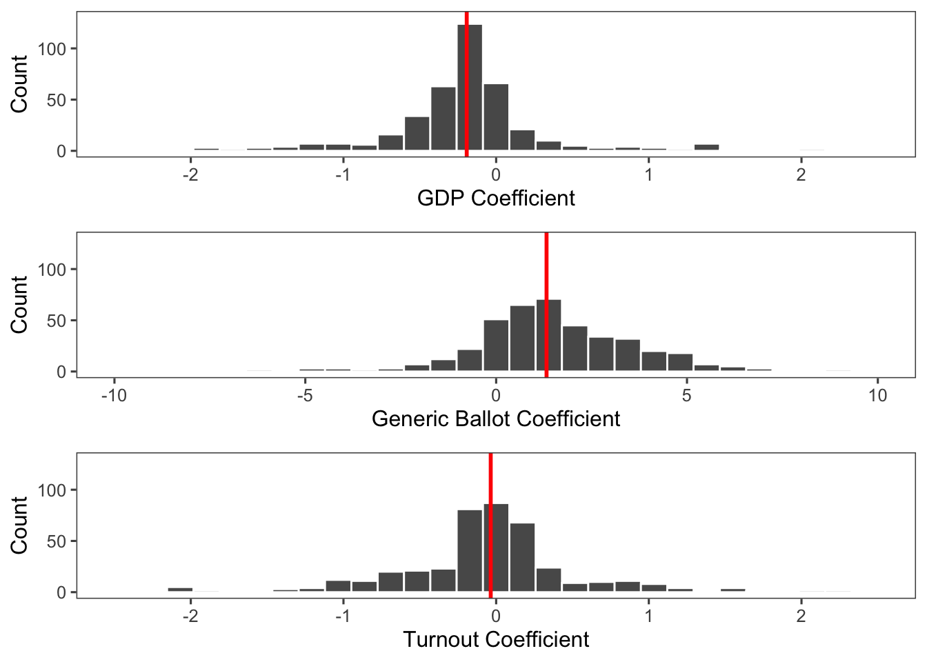
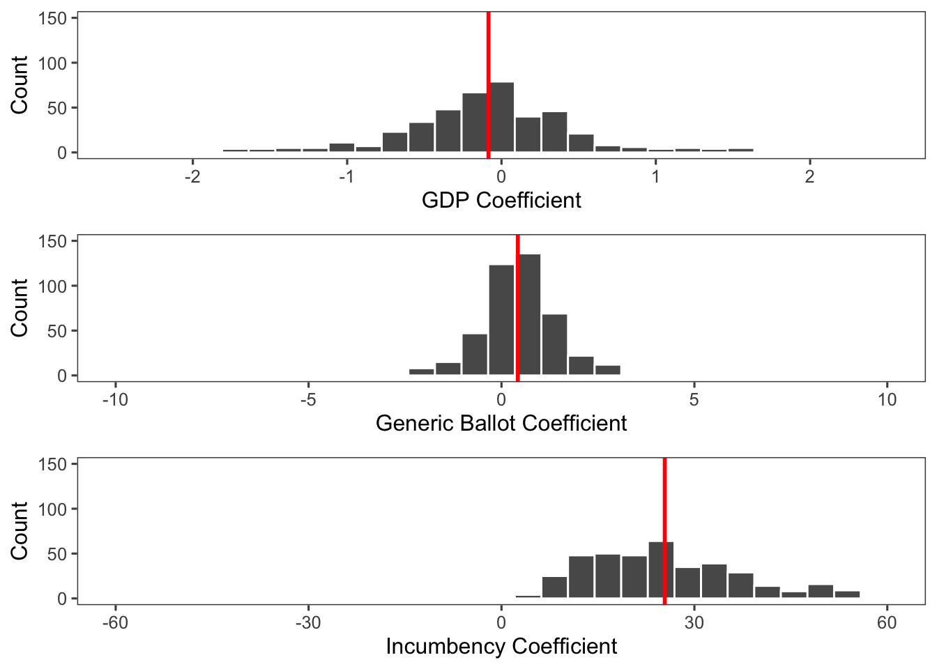
However, we can still learn some things from this model. Below are histograms of the coefficients for each variable across the 435 models. We can see that the median GDP coefficient is negative, so Democratic vote-share tends to decrease when GDP increases. As expected, the median generic ballot coefficient is positive, so as the polling average for generic Democratic support increases, Democratic vote-share also increases. The median turnout coefficient is very close to zero, indicating that there may not be an effect for turnout, or that it may just about cancel out across all the districts.
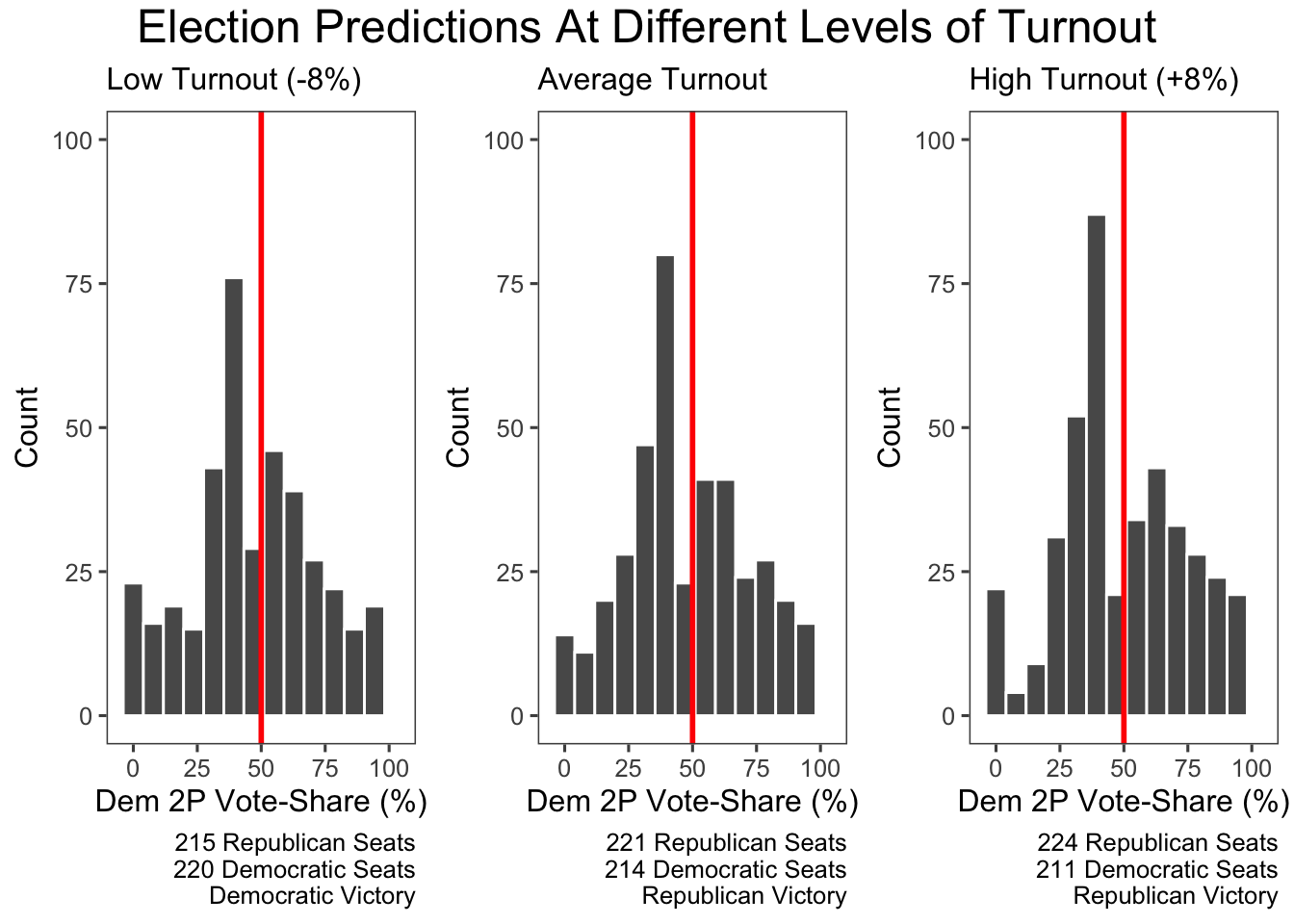
In order to make predictions with this model, we need to impute 2022 turnout information. I have attempted to guess what turnout will be like in 2022 by taking an average of turnout in 2014 (a very low turnout year), and 2018 (a very high turnout year). I then calculate a low, middle, and high turnout universe by adding/subtracting 8 percentage points of turnout, which we find as the maximum amount a campaign could move turnout (Enos and Fowler, 2016). Below are the results from predicting 2022 with our turnout model. From this, it appears that Democrats actually do better in a low turnout world, which makes sense with the recent shifting of more educated, high turnout voters to the Democratic Party.
Improving the Model
Of course, our previous model with turnout had many issues. Removing turnout will allow us to add more elections back into our model. In addition, turnout didn’t seem to have a very large effect - we only saw minor changes in the seat share when we increased or decreased turnout by the maximum amount in every district. So, we use the same model as before without the turnout variable. An example specification is below for our previous example of Wyoming:
\(~\)
| Example Regression Model | |||
| Wyoming | |||
| Characteristic | Beta | 95% CI1 | p-value |
|---|---|---|---|
| average_support | 0.84 | 0.29, 1.4 | 0.004 |
| gdp_percent_difference | -0.55 | -1.2, 0.10 | 0.094 |
| incumb | 8.9 | 1.6, 16 | 0.018 |
| Adjusted R² = 0.384; No. Obs. = 36 | |||
| 1 CI = Confidence Interval | |||
\(~\)
The model already looks better! All of the coefficients are significant, the adjusted r-squared is positive, and we’re actually able to predict based on incumbency since we have more years of data. In addition, the r-squareds of all the models looks better as well.
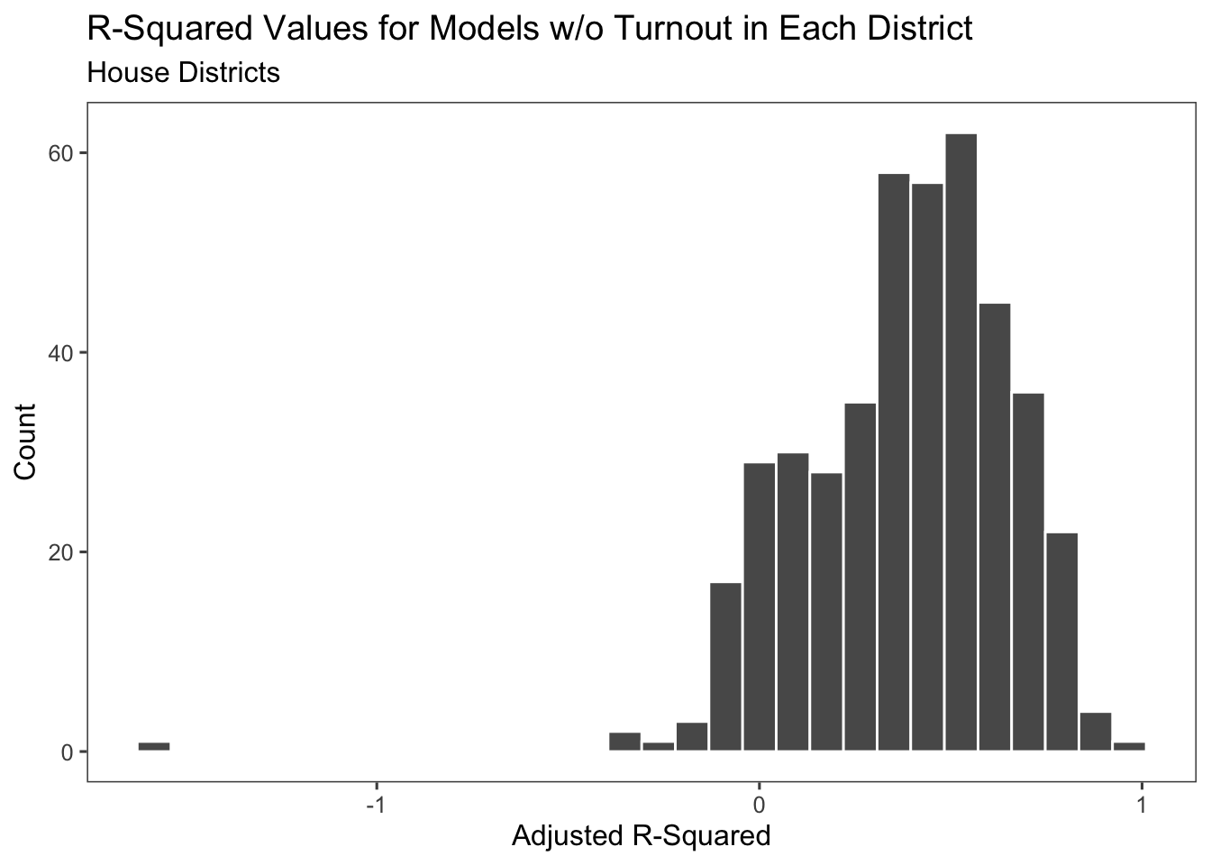
The median coefficents for GDP and the generic ballot are the same as those in the turnout model. Here, we’re also able to take a look at the incumbency coefficients. We can see that it’s massively positive, indicating that if you’re an incumbent in the district, your chances rise very sharply. This takes into account the fact that most districts are quite politically extreme and tend to always put Republicans or Democrats into office, regardless of various national conditions.
Final Predictions
Using our final model without turnout, we are able to make some predictions about the election. Below, we see the distributions of the predictions. This gives us 220 Democratic seats and 215 Republican seats, so the model forecasts a House majority for Democrats in 2022, though they will lose some of the seats that they currently have.
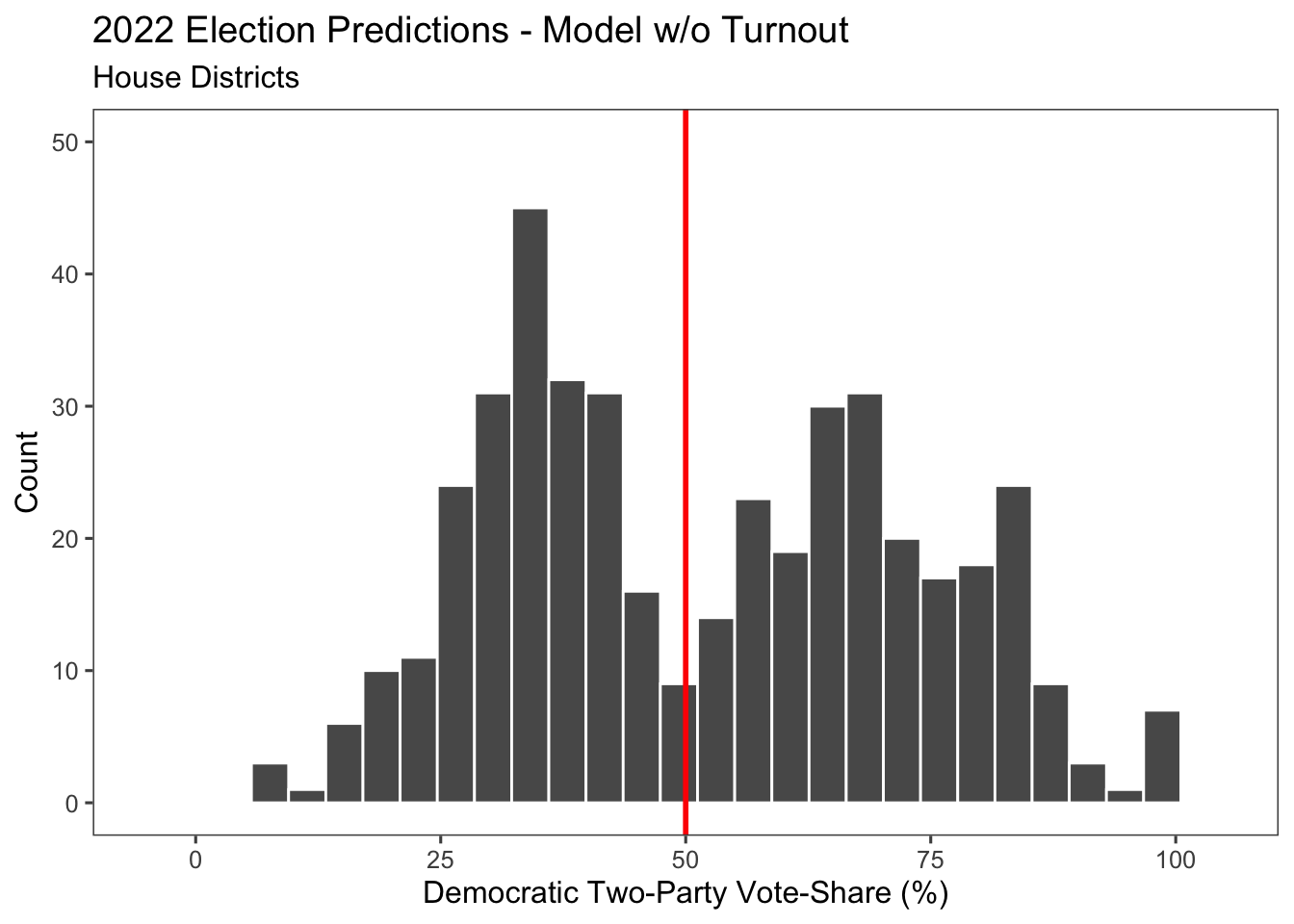
This model predicts the following flipped seats from 2020.
\(~\)
| Flipped Seats | |
| Seat | Predicted Party |
|---|---|
| Michigan-11 | R |
| Pennsylvania-1 | D |
| Pennsylvania-5 | R |
| Arkansas-4 | D |
| California-45 | R |
| California-49 | R |
| Florida-3 | D |
| Florida-27 | D |
| Illinois-14 | R |
| Virginia-10 | R |
\(~\)
This is an initial stab at building a model across every district. In the following weeks leading up to the election, I’ll continue to improve it.