on
Further Model Improvements (Week 7)
Introduction
Since we are now approaching the election, the primary focus for this week will be continuing to improve the model that I’ve been building week to week. My focus this week will be in exploring three major things. First, I look to improve the district-level model from Week 6 by adding an interaction term between the economy and incumbency as well as some other fundamental indicators for the districts. I then cross-validate this model using leave-one-out cross-validation on each model in each district. From this, I find that this model is overfitting and I look into exploring the usability of a pooled model of the districts.
District-Level Model Improvements
To my district-level model from last week, I’m adding a couple of changes. First, I’m adding an interaction term between incumbency and the economy. We know from Week 2’s exploration of the economy that academic theory and our own findings seem to indicate that voters punish the incumbent for a bad economy, so building it in as interaction can reflect that. In addition, I added indicators for which party currently held power in the House and which party currently held the presidency. I also added the Democratic vote-share in the previous midterm election for the party. Adding these variables improved the average adjusted r-squared of all of the district models in comparison to the one created last week. I’ve added an example specification of the model below.
\(~\)
| Example Regression Model | |||
| Wyoming | |||
| Characteristic | Beta | 95% CI1 | p-value |
|---|---|---|---|
| average_support | 0.66 | 0.05, 1.3 | 0.035 |
| gdp_percent_difference | -0.37 | -1.8, 1.0 | 0.6 |
| incumb | 9.7 | -1.1, 20 | 0.076 |
| house_party_in_power_at_election | -1.7 | -7.8, 4.4 | 0.6 |
| pres_party_in_power_at_election | -6.3 | -12, -0.35 | 0.039 |
| prev_results_dist | 0.26 | -0.11, 0.62 | 0.2 |
| gdp_percent_difference * incumb | 1.2 | -8.1, 11 | 0.8 |
| Adjusted R² = 0.420; No. Obs. = 34 | |||
| 1 CI = Confidence Interval | |||
\(~\)
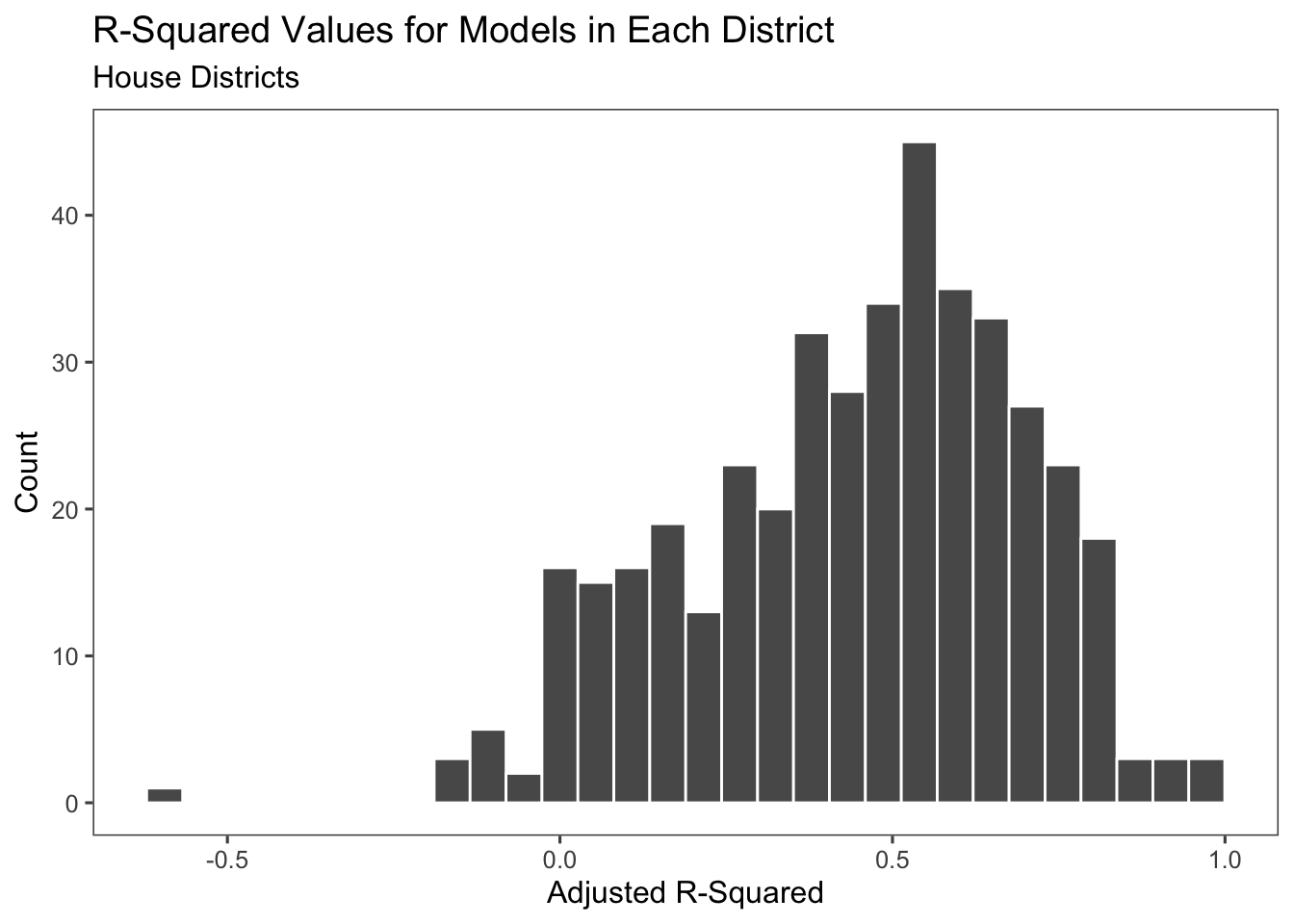
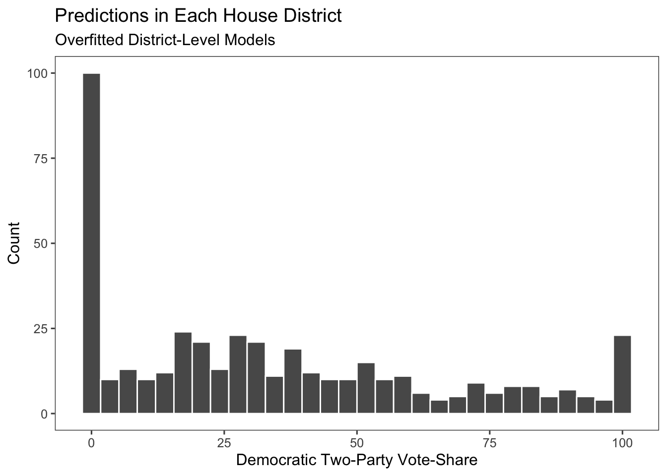
Adding these additional predictors, however, have created some issues with the predictions. The model is now giving a lot of negative values for the vote-share. The ultimate prediction also gives us 127 Democratic seats and 308 Republican seats, which seems a bit outlandish. This is a case where I believe that we have significantly overfit the model.
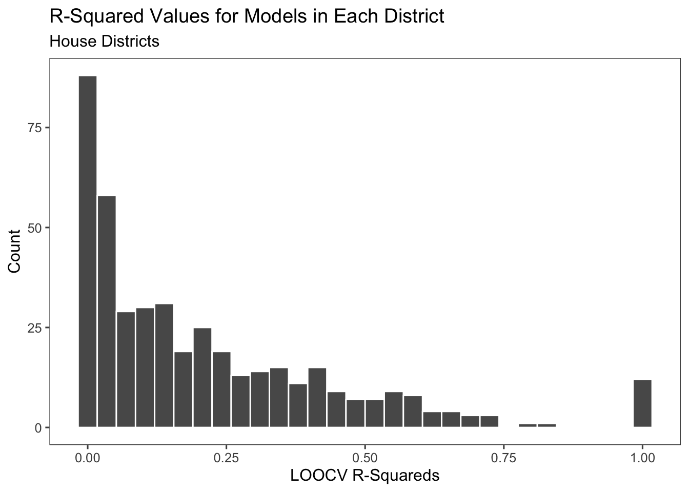
In order to test for overfitting, I use a method called leave-one-out cross-validation, where I remove one election from the training data set in order to test the model, and repeat this for all the elections. The results from this are significantly lower r-squareds for the model and indicate that there is overfitting in this model.
Pooled Model
Something else that I tried this week is a pooled model. This takes this districts and puts them all in one model to predict off of, instead of 435 different models. Below we can see that the model is significant for all of our predictors except for GDP alone and has a much higher adjusted R-squared. I also tested it with a bootstrap method and got a very similar r-squared value.
\(~\)
| Pooled Regression Model | |||
| Original Specification | |||
| Characteristic | Beta | 95% CI1 | p-value |
|---|---|---|---|
| average_support | 0.41 | 0.35, 0.46 | <0.001 |
| gdp_percent_difference | -0.04 | -0.13, 0.05 | 0.4 |
| incumb | 23 | 22, 24 | <0.001 |
| house_party_in_power_at_election | -2.7 | -3.2, -2.1 | <0.001 |
| pres_party_in_power_at_election | -4.8 | -5.3, -4.3 | <0.001 |
| prev_results_dist | 0.38 | 0.37, 0.40 | <0.001 |
| gdp_percent_difference * incumb | -0.15 | -0.27, -0.03 | 0.017 |
| Adjusted R² = 0.634; No. Obs. = 14,382 | |||
| 1 CI = Confidence Interval | |||
\(~\)
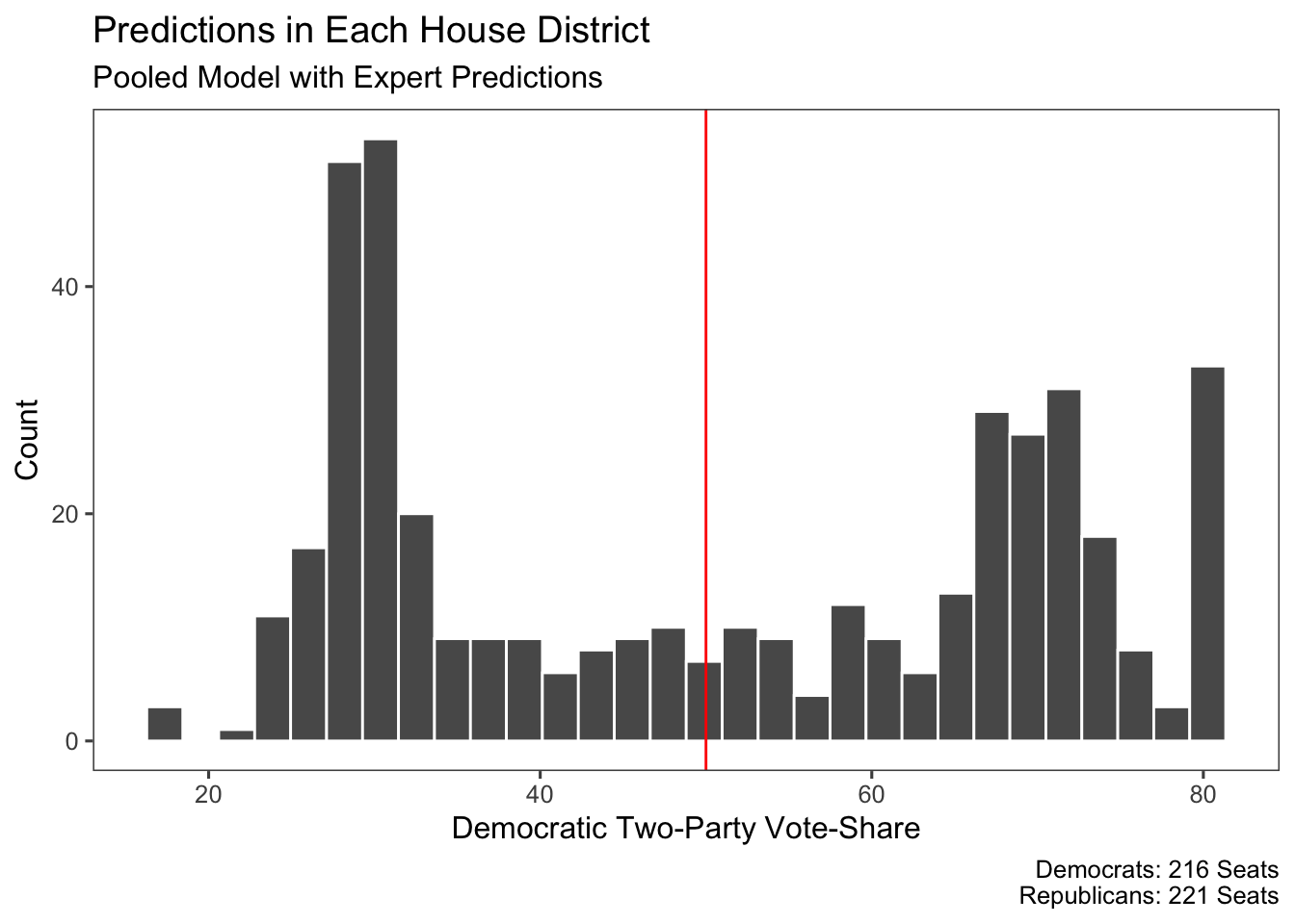
Unfortunately, however, our predictions end up a little wonky. Because our model relies very heavily on incumbency and previous vote share, it tends to not take into account center values and predicts very extreme districts outcomes.
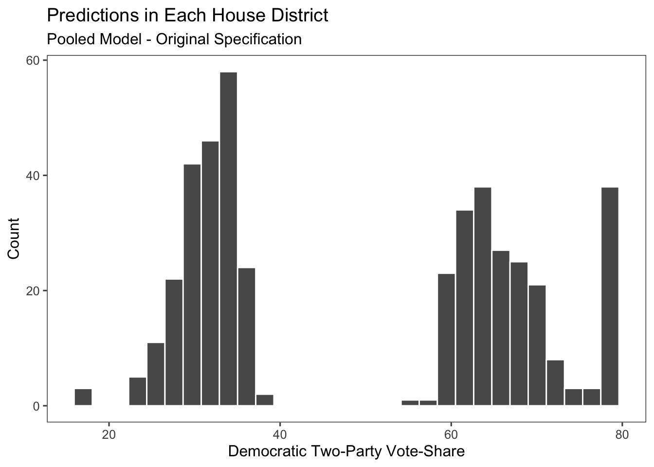
As an adjustment to the model, I instead include expert predictions. This cuts down on the number of years that we use in the model due to the limited nature of expert predictions, but it adds a bit more information for each individual district.
\(~\)
| Pooled Regression Model | |||
| Adding Expert Predictions | |||
| Characteristic | Beta | 95% CI1 | p-value |
|---|---|---|---|
| average_support | 0.28 | 0.23, 0.33 | <0.001 |
| gdp_percent_difference | 0.00 | -0.08, 0.07 | >0.9 |
| incumb | 3.3 | 2.4, 4.1 | <0.001 |
| house_party_in_power_at_election | -2.0 | -2.4, -1.5 | <0.001 |
| pres_party_in_power_at_election | -3.5 | -3.9, -3.1 | <0.001 |
| prev_results_dist | 0.33 | 0.32, 0.34 | <0.001 |
| avg_rating | -4.4 | -4.6, -4.3 | <0.001 |
| gdp_percent_difference * incumb | -0.22 | -0.32, -0.11 | <0.001 |
| Adjusted R² = 0.721; No. Obs. = 14,436 | |||
| 1 CI = Confidence Interval | |||
\(~\)
This change to the model did appear to improve the predictions and it looks closer to what could be an average distribution of the results could be. It’s not perfect, especially with the clustering of values around 30% and 70% Democratic vote share, but if we’re using it simply for classification purposes then this is alright.
Conclusion
\(~\)
| Final Predictions | |||
| Lower Bound | Prediction | Upper Bound | |
|---|---|---|---|
| Democratic Seats | 213 | 216 | 217 |
| Republican Seats | 222 | 219 | 218 |
\(-\)
The final predictions that we get from this model tell us that there will be 216 Democratic seats and 221 Republican seats, so Democrats will narrowly lose control of the House. The upper and lower bounds of this model are actually quite tight - they’re within five seats of each other and predict a Democratic loss either way. For my final improvements to the model next week, I will improve and test this model and add in redistricting data in an ensemble format.